It’s often useful to be able to visualise things in mathematics. For example, if you’re familiar with a function like \(x^2\), which squares whatever you put into it, you might already be imagining a plot of it on a pair of perpendicular axes, with two parabolic curves stretching upwards to each side.

Visualisations like this are easy when your function is one-dimensional: \(x^2\) takes one numerical input and gives one output, which means you can plot \(x\) on one axis and \(x^2\) on another to see how the latter changes as you vary the former. It’s a neat, compact visual representation of a function, and can be very useful if you’re trying to analyse how functions behave.

But if the functions you’re studying aren’t simple one-in-one-out functions, they might have multiple inputs and outputs. If your function is 2D, like this one:

\[f(x,y) = (x+y^2, x-2y)\]

then it’ll take in two inputs (\(x\) and \(y\)) and give you two values of output: in this case, one is given by \(x+y^2\), and the other by \(x-2y\).

For example, if you input the pair of values (0,0), this function would output (0,0), but if you put in (1,1) it’d give you (2,−1). These are just glimpses of how the function behaves – in order to get a full picture, like our graph of \(x^2\), we’d need to line up all the possible input values along an axis, and plot all the possible output values on another axis perpendicular to it – but this doesn’t work. Our input values are two-dimensional (and writing them as a pair of numbers in brackets is immediately evocative of points in a 2D plane), and so are our output values – so plotting these against each other would give a 4D graph.

This is difficult to visualise (if you can imagine a 2D plane, and then another one that’s at right angles to it, but not just in one direction – in both directions at the same time… no, it’s not working is it) and even harder to represent as a drawing on a piece of paper. Not even a 3D plot, or even a 3D physical model is enough to capture it.

So how do mathematicians visualise 2D functions like this? It’s difficult. If I create an applet that allows me to drag around a point and see what happens to its image under my function, you can see it moves around in an interesting way – but this is just a frustratingly tiny glimpse of the true story of this function.

Another way to analyse functions like this is to look at what happens to a set of points – for example, if we draw a simple shape like a circle or square in the plane, and then map each of the points in that shape to its image under the function, this gives us a crude picture of how this function distorts the plane. The image of a square under my function is a distorted curve, and a circle maps to a similar loopy shape.

These kinds of 2-dimensional functions are necessary if you’re studying complex numbers – this is a way to extend our usual notion of numbers to include some extra ones not usually considered to be numbers. They’re all based around the notion that you can’t usually take the square root of a negative number: nothing squares to give a negative number, as any number times itself, even if it’s negative, will give a positive result.

One way to get around this is to just define a new thing – we say that the letter 𝑖 represents the value of \(\sqrt{-1}\). Then, we can say \(i^2=-1\) and \(2i\) is the square root of \(-4\), and so on. This allows us to extend our usual one-dimensional real number line into a 2D plane, with a real axis running left-to-right with values \(1\), \(2\), \(3\) and so on, and an imaginary axis running top to bottom, with values \(i\), \(2i\), \(3i\) in the same way.

Any point in this plane represents a single number, denoted \(z=x+iy\), which means we can write functions in terms of 𝑧 and examine how they behave – but even though they have one complex input and output, we can’t draw them on a graph like we did with \(x^2\), since the input and output are both 2D numbers. While \(f(z)\) might look like a normal function, you always have to remember you’re working in the complex plane.

For example, the function \(f(z)=z^2\) is more complicated than \(f(x)=x^2\) was – we need to work out what ‘squaring’ means in this complex version; it’s not just squaring both coordinates. Since \(z=x+iy\), we have

\[ z^2 = (x+iy)(x+iy) = x^2 + 2ixy + i^2y^2\]

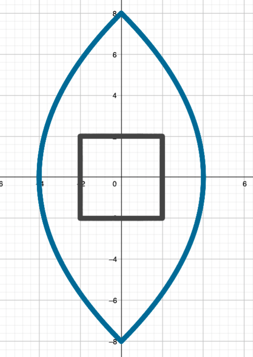
Since \(i^2 = -1\), this can be written as \(x^2 +2ixy – y^2\). This function can be interpreted as a 2D function – any terms with an \(i\) in them move things in the vertical direction, and any without \(i\) will affect the horizontal direction – so the function is effectively \(f(x,y)= (x^2-y^2, 2xy)\). It maps a square like this one to a lens shape, and this circle centered at (0,0) to another circle twice the size.

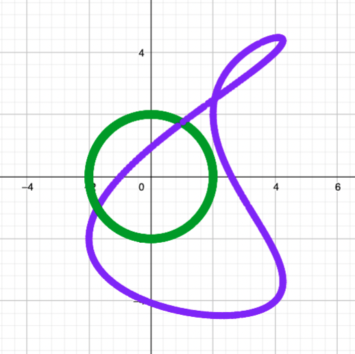
Let’s consider a different complex function: \(f(z)=z – \frac{1}{z}\). This takes a complex input \(z\), and maps it to \(z – \frac{1}{z}\). Seems simple enough! The coordinate functions here are slightly less simple – they work out to be \(\frac{x(x^2+y^2+1)}{x^2+y^2}\) and \(\frac{y(x^2+y^2-1)}{x^2+y^2}\). Let’s see what happens if I apply it to a circle.

The mild sense of intrigue you’re possibly now feeling was first felt by Russian mathematician Nikolay Zhukovsky back in 1910, when applying this transformation to a circle first resulted in this weird aerofoil shape. It turns out that for certain circles, this map will give you a perfect aerodynamic fin shape, very similar to those used in aeroplane wing design. If you change the size of the circle, it will change the thickness of the aerofoil, and the position of the circle affects the angle of the slope.

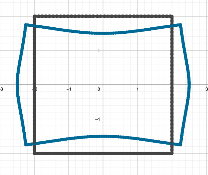
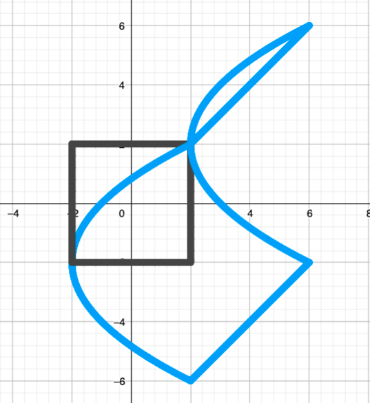
Another useful feature of this particular mapping is that it’s conformal almost everywhere in the plane – this means that it preserves angles. For example, if you’re mapping an object like a square, the image of this square under the map will still have four right-angle corners (even if they’ve been moved or the lines between them are curved) – this diagram (left) shows the image of a square under this map, called the Zhukovsky transform, and you can see it’s kept the right angles.

This means if you’re studying something like the flow of air around an object, and can find a way to describe that flow mathematically (e.g. as a vector field, showing how air is moving at each point in the space around it by attaching a vector at that point) you can look at the image of that flow under this map, and it will be transformed in a way that’s consistent, and tell you something useful about the flow around this new object.

Since the air flow around a cylinder is a well-studied phenomenon and we have equations to describe it, this allowed Zhukovsky to study air flow around wings whose cross-section looks like these aerofoil shapes, and describe it mathematically too. Performing complicated calculations like this was otherwise all but impossible before the invention of computers. In fact, Zhukovsky was the first scientist to study this type of air flow and explain the phenomenon of aerodynamic lift, and is sometimes called “the Father of Russian Aviation”.

Similar methods can be used to study other shapes of fin – for example, the Kármán–Trefftz transform gives aerofoils with a less pointy tail, using a different transformation function. Nowadays this kind of modelling is done using powerful computers – but Zhukovsky found that by visualising a function like this, you can apply what you know to something new. And isn’t that what maths is all about, really?