

Approximate Gaussian Elimination


One of the more technical lectures at the HLF so far was given by Daniel Spielman, on the Approximate Gaussian Elimination algorithm his research group has produced, and how it differs from traditional Gaussian Elimination. So what is Gaussian Elimination?
Described by Spielman beautifully as ‘the first recognisable algorithm’ that those studying maths and science learn, Gaussian Elimination is named after Carl Friedrich Gauss (strictly incorrectly, since the method was actually developed by Isaac Newton, and similar techniques appear in Chinese mathematical texts as early as 150BC).
Systems of Linear Equations
Gaussian Elimination is a way of solving a whole list of equations at the same time, that all deal with the same set of variables – for example, if you were given the following equations to solve:
5x + 5y – 4z = 0
8y – 3z = 9
z = 5
It would be obvious that you could immediately substitute this exact value for z into the second equation to get an exact value for y (in this case, the equation becomes 8y – 15 = 9, so 8y = 24, so y = 3). You could then substitute these values for y and z into the first equation, so that 5x + 15 – 20 = 0, hence 5x = 5 and x=1.
So, if a set of equations has this nice easy property that each only includes one variable we don’t already know, we can find a solution with very little effort. However, most equations in the real world don’t behave like this, and you’ll often find some things depend on all of the variables in a way that this kind of approach can’t immediately help with. For example:
9x + 3y + 4z = 7
4x + 3y + 4z = 8
x + y + z = 3
A Process of Elimination
In Gaussian elimination, the aim is to eliminate some of the variables, thus leaving us with a simpler set of equations. The key is to recognise that with these types of linear equations, we can perform simple linear operations to change the equations, without breaking the system.
For example, if we know x + y + z = 3, it’s obvious that 9x + 9x + 9z = 27 – we can multiply the whole equation by 9 and it retains its correctness. Even better, we can combine the equations by adding one, or a multiple of one, to another.
In our previous example, when we substituted in a value for z into the equation above it, we were essentially taking -3 times that equation and adding it to the equation above – this cancels out the -3z in the previous equation, eliminating it from the system.
Using this method, we can apply the same technique to simplify our more complex system of three equations (let’s label them, for convenience).
A: 9x + 3y + 4z = 7
B: 4x + 3y + 4z = 8
C: x + y + z = 3
For example, we could take equation C, multiply it by 9, and subtract it from equation A to eliminate the x term, giving:
A: -6y – 5z = -20
B: 4x + 3y + 4z = 8
C: x + y + z = 3
Then, we could subtract 4 times equation C from equation B, to give:
A: -6y – 5z = -20
B: -y = -4
C: x + y + z = 3
Now we’re left with a set of three equations, which includes an exact value for y, an equation in y and z we could use to get a value for z, and an equation in all three we could then use to find x.
Enter The Matrix
This process can be used for any size of set of equations – although in practice, instead of using equations written out in variables like this, the coefficients in the equations are placed into a matrix A, and the variables and solutions into vectors x and B. The matrix and vectors are then related by an equation:
Ax = B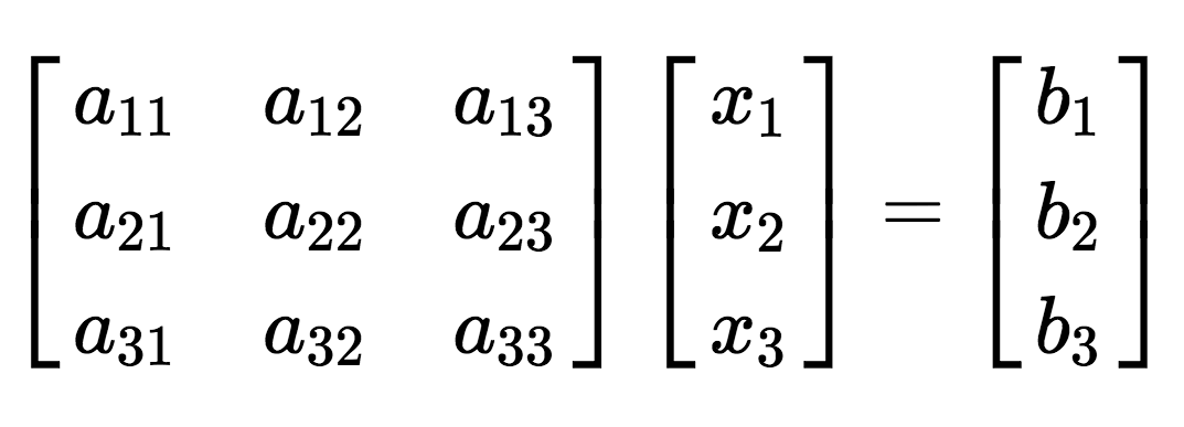
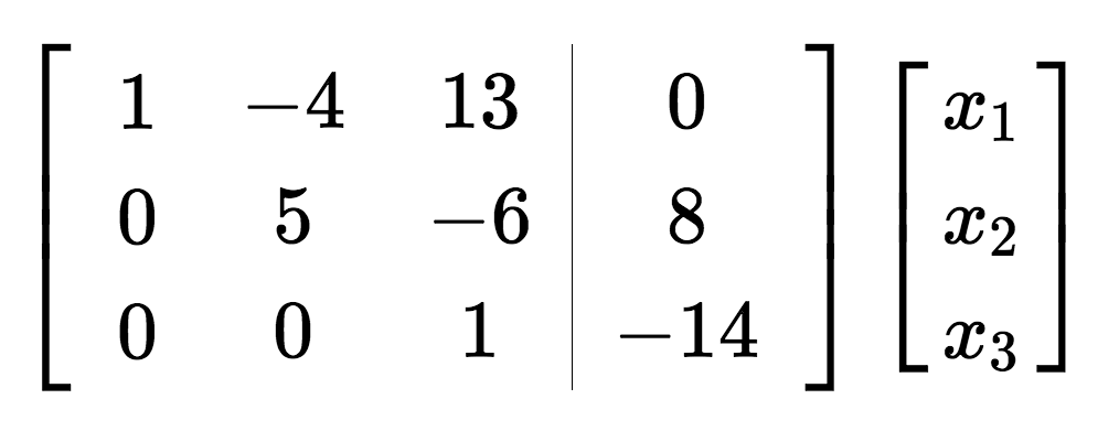
To perform the elimination, the vector of solutions is appended to the right hand side of the matrix to give the augmented matrix, and then row operations (adding together linear combinations of the rows) can be performed on the matrix more easily by computer.
The goal is to achieve a matrix with zeroes in the whole of the lower left region, known as an upper triangular matrix, also known as a matrix in row echelon form. Solutions to the family of equations can then be easily computed.
 The process of Gaussian Elimination can also be used to perform many other operations on matrices – finding the determinant, inverting the matrix, or computing the rank. It’s used in applications across maths and computer science, for matrices with up to thousands of rows and columns.
Efficiency Savings
Gaussian Elimination is undoubtedly effective, but not always super-efficient. Computing with large matrices can be very slow. The number of operations needed to put a matrix in row echelon form is around n3 for an n by n matrix, and as n grows large this takes a long time. More efficient methods are available though, and one was described by Spielman in his talk.
Approximate Gaussian Elimination uses techniques which aim to reduce the number of non-zero entries in the matrix – as it’s then possible to perform the elimination using fewer computer operations, as many more of the calculations will be zero. The method however doesn’t give a precise answer, as in creating all the extra zeroes, some of the values in the matrix need to change slightly.
However, this doesn’t mean the method can’t be used to produce accurate results – once an approximate solution is achieved, the residual can be computed, and the process repeated to get closer to the actual answer. This means within a few iterations the method will produce an answer sufficiently close to the result.
The method is also particularly suited to calculating with Laplacian matrices – matrices which represent the structure within a graph or network – as the way the elimination works gives another matrix which is the Laplacian of a similar graph, and the changes made to get from one graph to the other can be simply described.
Spielman presented a table of computation times which show that their method, for certain types of calculations, outperforms the existing widely-used methods dramatically. He also stressed that one nice benefit of the Approximate Elimination method is that the amount of time it takes is consistent across many different types of problem. This means it’s especially suited to being used as a subroutine within a larger programme, as it’s easy to predict how long it’ll take, and you won’t risk slowing down your programme waiting for it to finish.
The only thing Spielman regrets is that no exciting mathematical theorem has yet been proved about this new algorithm – it’s always a satisfying result when this can happen, and he hopes it’ll be forthcoming in the near future.
The applications of this type of mathematics are endless, and as algorithms like this become more and more efficient, it’s a lovely example of how maths and computer science can productively collaborate!
More information
Daniel Spielman’s entry on the HLF website
Approximate Gaussian Elimination for Laplacians: Fast, Sparse, and Simple – paper by Spielman’s colleagues Syng/Sachdeva, on the ArXiV
Laplacians.jl, Spielman’s Julia code for manipulating Laplacians, on GitHub
Approximate Gaussian Elimination for Laplacians: Fast, Sparse, and Simple ends with the following Acknowledgements: We thank Daniel Spielman for suggesting this project and for helpful comments and discussions.
I know Gaussian Eliminaton since I studied 40 years ago. I just know, that in case of tridiagonal Matrix the calculation need not so much calculations. But I know, that there some ways of approximation.