Algorithms and Life

We tend to think of algorithms and computation as human inventions, but organisms as primitive as bacteria have relied on algorithmic mechanisms throughout the history of life. The regulation of genes inside a single cell, feedback loops in the control of metabolism, the coordinated motions of bird flocks, and the foraging behavior of social insects: All these phenomena can be succinctly described in an algorithmic framework. Another notable example is pattern formation in animals—the tiger’s stripes and the leopard’s spots—for which Alan Turing proposed an algorithmic mechanism in 1951.

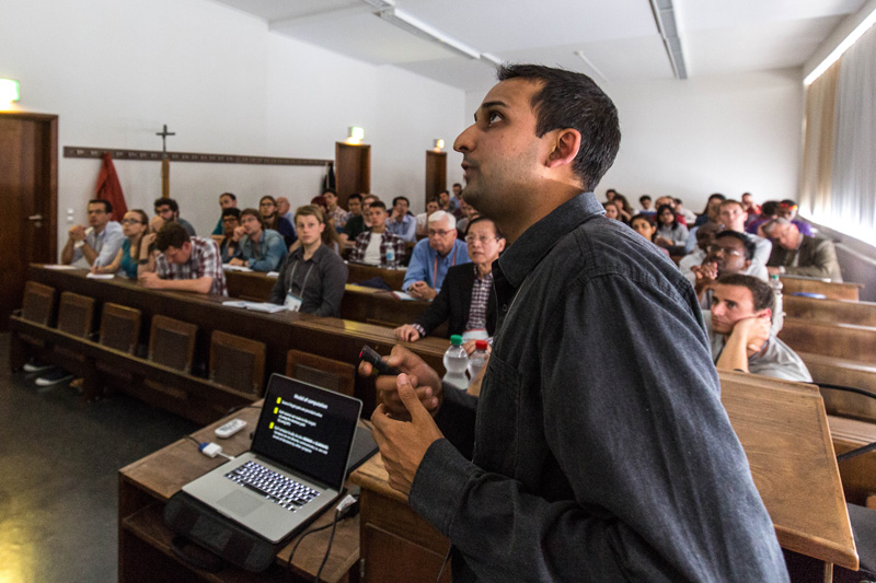
“Algorithms in Nature” was the title of a postdoc workshop presented Tuesday by Saket Navlakha, who is an assistant professor at the Salk Institute and one of the 200 young researchers attending the Heidelberg Laureate Forum. With Ziv Bar-Joseph of Carnegie Mellon University, Navlakha maintains a website on the same theme; they were also co-authors of a survey article on these ideas published in January in Communications of the ACM.

If we look upon living organisms as computational mechanisms, what kind of computer systems are they? Navlakha points out that they are often distributed systems, with many processing elements and no central governing authority. For example, some species of fireflies synchronize their flashing, and they must do so without having a designated leader to keep the beat. Another distinctive characteristic of many biological algorithms is a random or stochastic component. The randomness is not just unavoidable noise; it can be advantageous in the Darwinian contest with predators, parasites, or rivals, just as it is in computer algorithms for cryptography and other adversarial contexts.

After a brief survey of biological algorithms, Navlakha turned to his work on the development of connection patterns in the network of neurons, or nerve cells, in the mammalian brain. The connections consist of the specialized junctions called synapses, where one neuron touches another, allowing signals to jump from cell to cell. The set of interconnected neurons forms an immense network. In the human brain there might be 10¹¹ neurons and 10¹⁴ synapses.

The mammalian brain does not have a full complement of synapses at birth. In human infants the number of synapses and the density of connections increases rapidly until about age two, bringing more neurons into direct contact with one another. Then something surprising happens: The number of synapses begins to decline again. New synapses continue to form, but even larger numbers are abandoned and eliminated. The neural network is “pruned,” like an overgrown shrub. Eventually the number of synapses drops by 50 or 60 percent from the peak at age two.

This loss of synapses is not a sign of atrophy or deterioration; neurophysiologists believe it is a normal phase of development and is associated with learning. A sensory pattern—something you see or hear, perhaps—stimulates activity along a particular set of neural pathways. If a pattern appears frequently, synapses along the corresponding pathways are strengthened, whereas those that are seldom stimulated are pruned away. Evidence supporting this hypothesis came from experiments done in the 1960s by Torsten Wiesel and David Hubel, who found that signal pathways between the eye and the brain obey a “use it or lose it” protocol.

However, a puzzling question remains: Why expend the energy and other resources needed to build a densely interwoven network, then throw away half the connections? Wouldn’t it be more efficient to start from a sparsely connected initial state and add synapses only as needed?

Navlakha and his colleagues examined this question with a model that reduces the intricate geometry of brain cells to an abstract mathematical graph—a network of nodes and edges, where the nodes represent neurons and the edges represent synapses connecting one neuron to the next. Diagrammatically, the graph is a collection of dots (the nodes), with lines or arrows connecting them (the edges).

Many algorithms for “growing” such networks have been studied in the past 60 years. In a scheme first described by the mathematicians Paul Erdős and Alfred Renyí, you begin with a set of isolated nodes, with no connecting edges. Then a random process is applied repeatedly: You choose two nodes at random and flip a coin to decide whether or not to draw an edge between them. In a variant algorithm called preferential attachment, a node is more likely to acquire new edges if it already has a large number.

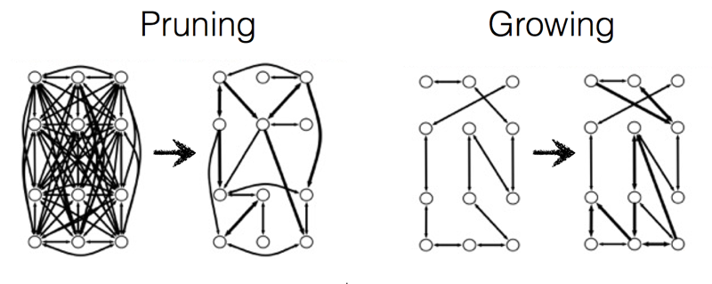
A distinctive property of these graph-growing algorithms is that they only add edges to the graph; they never remove them. Navlakha and his colleagues experimented with an alternative, subtractive, process in which the graph is shaped by pruning edges rather than sprouting new ones. They started with a fully connected graph (a “clique”), in which every node is linked to every other. Signals were then repeatedly routed through the graph between randomly selected pairs of nodes. Of the many routes available between any two nodes, they chose either the shortest route or a route that was found by an algorithm called breadth-first search. Each edge kept track of the number of times a signal passed through it. After a training period, edges that failed to reach a threshold of popularity self-destructed. In this algorithm the network is reconfigured by strictly local actions. Each edge in the graph (or each synapse in the neural network) makes its own life-or-death decisions, without any need for a central controller or even for communication between synapses.

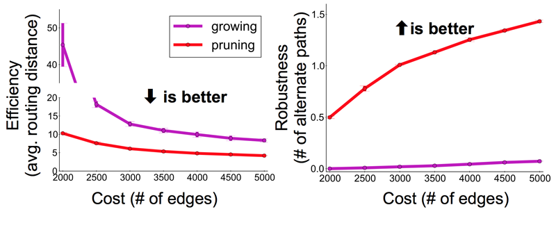
Navlakha and his colleagues compared two properties of graphs formed by subtractive vs. additive algorithms. They looked at efficiency, measured as the average number of edges that have to be traversed to connect two randomly selected nodes. They also looked at robustness, expressed as the average number of alternative paths between two nodes; a more robust network is less likely to be split in two by the loss of a single edge. By both measures the subtractive networks turned out to be superior to the additive ones. In comparing graphs with the same number of nodes and edges, the pruned networks were consistently more efficient and more robust. Navlakha notes that this comparison is based purely on the structure of the networks, and may or may not extend to their functional suitability for neural processing.

A further question now arises: What is the optimal schedule for pruning? If you wait until late in the training process, you get the benefit of more data and thus might make more accurate judgments about the utility of each synapse. On the other hand, the late-pruning strategy comes at a metabolic cost, expending energy to maintain a population of synapses that are not in fact needed. Navlakha consulted the neurobiological literature to find out how real neural networks develop over time, but he found that the necessary experiments had not been done. So he undertook to do them himself!

By education and experience, Navlakha is a computer scientist, but in collaboration with biologists he conducted a year-long laboratory project to profile the timing of the pruning process in the mouse brain. They looked at a particular site in the brain, one that receives signals from one of the mouse’s whiskers (an important sensory input in rodents). Mice were raised to a certain age, then sacrificed, and the selected brain tissue was sliced with a microtome into sections 50 microns thick. The sections were stained with a reagent that makes synapses more conspicuous, then imaged with an electron microscope. To analyze the images and count the synapses, Navlakha built a machine-learning system based on a support vector machine, a computer program that classifies images according to features it has been trained to recognize—in this case the characteristic textures and shapes of synapses.

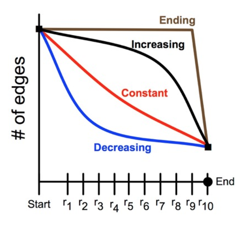
The brain tissue was examined at 16 stages of development, ranging from 14 to 40 days after birth. (Mouse brains develop much faster than human brains.) The study employed about 40 animals, generated almost 10,000 electron micrographs, and identified more than 20,000 synapses. Analysis of the data showed clearly that synapse-pruning follows a concave-upward trajectory: The number of surviving synapses declines quickly at the outset, but then the rate of loss diminishes, approaching a steady state where the number of synapses is constant.

Why would this decreasing-rate strategy be favored by natural selection? As noted above, there may be energetic advantages to early pruning, but Navlakha cites other factors as well. Hasty decisions about which synapses to eliminate may lead to a form of “overfitting,” in which the system gives too much weight to a few early data points. Also important is the distributed nature of the computation. Suppose that two synapses provide alternate, redundant pathways between the same neurons; efficiency demands that one synapse or the other be eliminated, but not both. A central coordinator could make the choice without difficulty, but a distributed algorithm drawing only on local information must be more cautious or risk partitioning the network.

Having brought a computer-science perspective to a problem in biology, Navlakha and his colleagues have also turned around and applied the findings in other computational realms. For example, they have tested the pruning algorithm on the task of designing airline routes in a network of 122 cities. Providing direct flights between all pairs of cities (there are more than 7,000) is not feasible, and so some travelers must make multiple “hops.” The aim is to minimize the average number of hops for a given total number of flight routes. Navlakha et al. found that pruned graphs were more efficient for this task than grown graphs, and among the pruned graphs the best performance came from a decreasing-rate pruning schedule.

For more details on this work see: “Decreasing-Rate Pruning Optimizes the Construction of Efficient and Robust Distributed Networks,” by Saket Navlakha, Alison L. Barth, and Ziv Bar-Joseph, PLoS Computational Biology, July 28, 2015, DOI: 10.1371/journal.pcbi.1004347.